12 on 12 Analysis » Do It Yourself

Variable Inputs

Step 1:

Insert Variable name into the “Variable 1” cell and the “Variable 2” cell found on the 2nd tab of your Excel template (E2). These variables are those that you deemed key indices to evaluate your sales.

Step 2:

Input time periods and their values into the first two columns in the table. For the time periods, creating monthly values as this will create your month over month change.

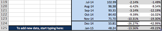To add new data, start typing in Cell E124 of the template. These cell numbers will change according to how many values you choose to measure.

Step 3:

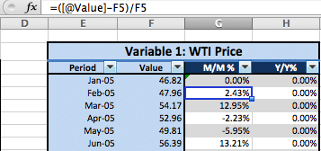In the M/M%, put 0% as your first percentage. For every percentage point below that row, put in this function:

=([@Value)-F5)/F5

This basically takes the current value, subtracts the previous value, and then divides it by the previous value. Continue doing this until you’ve completed the M/M% for every value you provided.

Step 4:

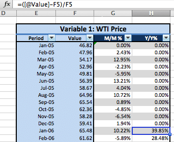
Now, it’s time to complete the Y/Y%. First, skip 12 months down. You will be starting at the beginning of Year 2.

Utilize the same function as before:

=([@Value)-F5)/F5

This time, you will be using the current value (first month in Year 2) subtracted by the first value listed in Year 1 and divided that by the first value listed in Year 1.

Continue to do this until you reach the end of your values. There should be a whole year of values that are not measured in this column.

Evaluate Changes

It’s time to start evaluating your variable inputs graphically. There should be 3 graphs that you want to to produce to increase your chances of catching trends and correlations: Absolute Value, Month over Month Change, and Year over Year Change.

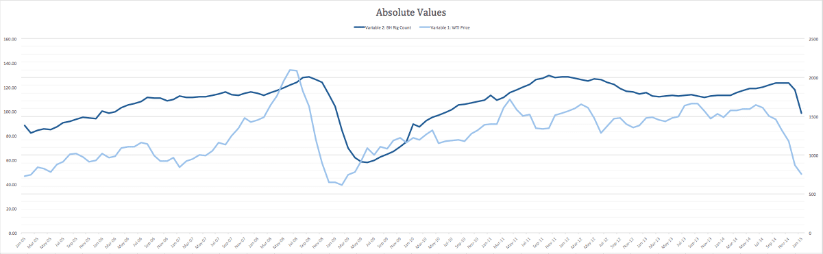
By calculating the absolute value, you’re able to see the full valuation of a company in relativity to those key variables you just choose. As you can see with this example, the rig count followed the WTI price closely. While the WTI price varied more frequently, the rig count stayed consistent (which makes sense because it’s difficult to build and dispose of rigs in any given day… It takes time).

You can also notice that the rig count is about 6 months behind the rise or fall of the WTI price. This is important to take note and track! This direct correlation can allow you to create more effective projections for your bank.

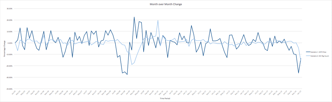
Again, you can see that the WTI price wavers more frequently and sharply than the rig count. A month over month change is useful so you can immediately adjust while still knowing that drops or rises in WTI price is completely normal.

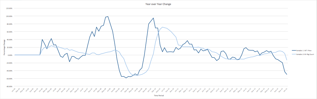
Your year over year change is incredibly useful when looking at your projections for the next year. Rig count still doesn’t fluctuate the same as WTI price, but it does still impact rig count.

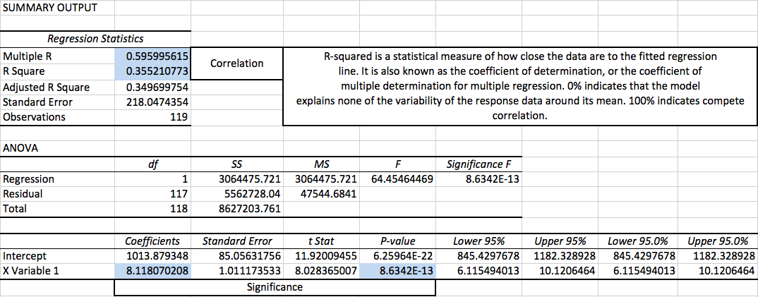
Summary Output

Now that you’ve calculated your variables and evaluated changes graphically, it’s time to compile all that data into a simple summary output. It’s important create statistical data from both internal and external variables to be effective as an economic and predictive analysis tool.

Regression Statistics

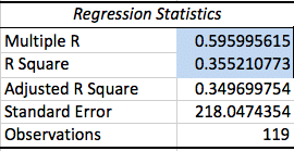R-squared is a statistical measure of how close the data are to the fitted regression line. It is also known as the coefficient of determination, or the coefficient of multiple determination for multiple regression. 0% indicates that the model explains none of the variability of the response data around its mean. 100% indicates compete correlation.

R = b0 + b1X

R is the link between both predicted and observed values.

R² = Regression SS / Total SS

R Square is the fraction of variability.

Adjusted R² = 1 – {[(1-R²)(N-1)]/[N-p-1]}

Adjusted R-Squared assumes that every independent variable explains the variation found with the dependent variable.

Standard Error = √Residual mean Square

The Standard Error is the standard deviation of the sampling, particularly on the mean.

ANOVA

ANOVA is short for Analysis of Variance, is an extension of the t- and z-tests. It created a way to test for several null hypotheses simultaneously by splitting the data into two categories: systematic factors and random factors.

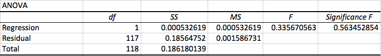
Regression SS is the variability accounted for by a particular regression model. The Residual SS is the difference between the Regression SS and the Total Sum of Squares.

df = degrees of freedom, n – 1

Degrees of Freedom is about means rather than single observations. The value of df is entirely dependent on the design of the test you’re conducting.

Total SS = Σ(yi – ymean)²

Sum of Squares describes how the response variable (Y) varies.

MS = SS / df

Mean Squares is the Sum of Squares divided by their respective Degrees of Freedom.

F = MSB / MSW

The F Test is utilized to test whether 2 variances are equal to one another. If the null hypothesis is true, F should be expected to have a value close to 1.0. A large F ratio typically means that the variance is more than originally expected.

To learn more about ANOVA, click here

Absolute Value Summary

As a refresher, absolute value is a valuation method that utilizes future free cash flow analysis to conclude the financial worth of a company. Absolute value has the ability to calculate the entire business’s worth. This is particularly important when considering selling the business or bringing on outside investors.

Month Over Month Summary

Month over month displays the difference in price or rig count in comparison to the previous month. The following statistics quantify the volatility of your key variables; therefore, it shows you the impact it will have on your company.

Year Over Year Summary

Year over year displays the difference in the key variable. This is in comparison to the previous year.

[gravityform id=”45″ title=”true” description=”true”]